|
Click here
to look at the table of assumptions used. Click here to view a cross-section explanation |
Gravity models are used to aid in defining major geologic features. All earth materials influence gravity measurements. However, the bulk of the Earth’s gravitational force has little to do with crustal rocks. Only about 0.05 percent of the gravitational force is contributed by the upper 8 miles of crustal rock (Grant, 1965, p. 190). Most important is the fact that this very small contribution can be detected by gravity meters and accordingly mapped. Gravity measurements must be subjected to a series of reductions and corrections before they are suitable for interpretation of geologic features.
Gravity variations are measured in gals; one gal is equivalent to a force of acceleration of one centimeter per second per second. The Earth’s average gravitational force is about 980 gals. Owing to the very small magnitude of variations measured, milligals (1/1,000 of a gal) are used for computational purposes.
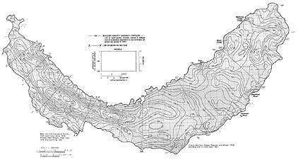
The above Bouguer gravity anomaly map is a summation of all gravity effects in the area. Corrections for most major non-geologic effects are incorporated in the map.
Because interpretations are non-unique, gravity modeling was used only as a guide to help define major geologic features where no other definitive data were available.
The modeling program is based on a two-dimensional polygon method (Talwani and others, 1959). The program uses polygons of varying sizes, shapes, and assumed density contrasts (table of assumption of density values) to represent possible geological bodies inferred from available information.
The following assumptions were made: (1) Subsurface density variations are modeled using polygonal bodies of infinite strike length; (2) each polygon is of a constant assumed density contrast (compared to an average for crustal rocks of 2.65 grams per cubic centimeter [see table of assumption of density values); and (3) compaction of material with increasing depth of burial is negligible.
The polygon’s gravitational effects are calculated in the program and a summation of these effects is plotted against the measured residual gravity anomaly.
Polygons are changed, deleted, or added as necessary to comply with known geologic and physical constraints until a best fit between the gravity field curve and the theoretical curve is obtained.
Gravity modeling of the western plain was done using Bouguer anomaly values obtained directly from the map. Modeling of the eastern plain required that the Bouguer anomalies be adjusted to compensate for the regional effects of a large body of rock either more aerially extensive than the pIain or deeply buried (more than 3 miles) under the plain (Mabey, 1978, p. 557). Data from a seismic refraction study (Sparlin and others, 1981, p. 53) suggest that the latter hypothesis is most likely correct.
These data were used as a basis for the regional residual separation. The separation was made using several methods suggested by Dobrin (1952, p. 86-88). Actual modeling extended beyond the plain’s boundary, but results shown in sections X-X’ through EE-EE’ are only for that part within the boundary. Sections were simplified because, in the modeling process, the ability to simulate several rock units of different densities exceeds present understanding of the subsurface distribution of rock units in the study area.
Delineation of major rock types by gravity modeling was marginally successful but did aid in understanding the regional structure. Seismic section J-J’ and gravity section Y-Y’ show good agreement in delineation of the sediment and Tertiary (Miocene) basalt unit contact.